Have you ever found yourself staring at a spreadsheet filled with rows of data, wishing you could quickly isolate specific information based on color? Perhaps you’ve color-coded cells to highlight important values or categories, but filtering through them manually feels like an impossible task. Fear not! Excel offers a powerful built-in feature that allows you to filter data by cell color, saving you time and effort.

Image: learnexcel.io
In this comprehensive guide, we’ll delve into the world of color filtering in Excel, exploring its functionalities and the various ways it can streamline your data analysis. From basic filtering techniques to advanced custom filters, we’ll cover everything you need to know to master this skill and unlock the full potential of your spreadsheets.
Understanding Color Filtering in Excel
What is Color Filtering?
Color filtering in Excel is a handy tool that allows you to quickly display only the rows in your spreadsheet that have cells with a specific color. This feature comes in handy when you’ve color-coded your data to represent different categories, priorities, or statuses. For example, if you have a list of clients and you’ve colored cells with red to indicate overdue invoices and green to signify paid invoices, you can use color filtering to easily see which clients have unpaid balances.
Why Use Color Filtering?
The beauty of color filtering lies in its simplicity and efficiency. It enables you to:
- Visualize data: Highlight key data points or patterns within your spreadsheet.
- Analyze data quickly: Filter out irrelevant information and focus on specific data sets.
- Improve decision-making: Gain valuable insights by analyzing color-coded data.

Image: excelchamps.com
How to Filter by Color in Excel
Excel offers two primary ways to filter data by color: using the standard filtering feature and through advanced custom filters.
1. Filtering by Color Using the Standard Filter
This method is the most straightforward and can be utilized for quick and easy filtering.
- Select the data range: Click and drag to select all the cells you want to filter. This should include the header row that contains the column names.
- Activate the Filter feature: On the “Data” tab in the Excel ribbon, click “Filter.” You’ll notice small drop-down arrows appear next to each column header.
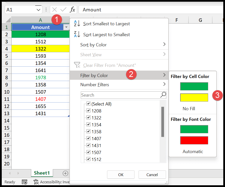
- Filter by Color: Click the drop-down arrow in the column you want to filter by color. You’ll see a list of options. Choose “Filter by Color” and then select the desired color from the submenu.
- Apply the filter: Excel will immediately filter the data, only showing rows with cells matching the selected color.
2. Advanced Color Filtering with Custom Filters
If you require more intricate filtering criteria or need to combine color filtering with other filter options, you can utilize custom filters. While this method offers greater control, it involves using more advanced filtering parameters.
- Select the data range: Follow step 1 from the standard filtering method.
- Activate the Filter feature: Follow step 2 from the standard filtering method.
- Open the Custom Filter: Click the drop-down arrow in the column you want to filter by color. Choose “Text Filters” and then select “Custom Filter.”
- Create the Filter Criteria: You’ll see two drop-down menus:
* **”Cell Color”:** Here, you can select the desired cell color.
* **”Font Color”:** This option allows you to filter by font color instead of cell color.
* **”Other options”:** You can combine these criteria with other filtering options like text values or numbers. - Apply the filter: Click “OK” to apply the custom filter.
Tips and Expert Advice for Color Filtering
Here are some expert tips to help you get the most out of color filtering in Excel:
- Consistent Color Coding: Maintain a standardized color coding system across your spreadsheets to ensure consistency and easy understanding.
- Use Color Legends: Add a legend to your spreadsheet or accompanying documentation explaining the meaning of each color.
- Combine Filtering Options: Don’t be afraid to experiment with combining color filtering with other filtering options like text or number filters to pinpoint data more effectively.
- Color Formatting Tools: Utilize Excel’s built-in color formatting tools like conditional formatting to automatically color cells based on specific criteria, making your data analysis even more dynamic.
- Remember the Filter Reset: Once you’ve applied a color filter, you can easily reset it by clicking the drop-down arrow in the column header and choosing “Clear filter from ‘column name.'”
Frequently Asked Questions
Here are answers to some commonly asked questions about color filtering in Excel:
- Q: Can I filter by cell color that was applied manually?
- A: Yes, you can filter by the color of cells that were manually colored. Excel doesn’t differentiate between colors applied automatically or manually.
- Q: Is there a way to filter by multiple colors simultaneously?
- A: No, you cannot filter by multiple colors at the same time directly using standard filters. However, you can create custom filters for each color individually.
- Q: Can I automatically apply color filtering based on specific criteria?
- A: Yes, you can use Excel’s conditional formatting feature to apply color to cells based on criteria like values, dates, or text content. This allows you to automatically trigger color filtering based on your specified conditions.
How To Filter By Color In Excel
Conclusion
Color filtering in Excel is a simple yet powerful tool that can streamline your data analysis and make your spreadsheets more visually engaging. By mastering this technique, you can easily identify and analyze specific data points, saving time and effort while gaining valuable insights into your data sets. So go ahead, experiment with color filtering and discover a new level of efficiency in your Excel endeavors!
Are you ready to unlock the power of color filtering in Excel? Tell us about your experience using this feature and any challenges or successes you’ve encountered. We’d love to hear your thoughts!


