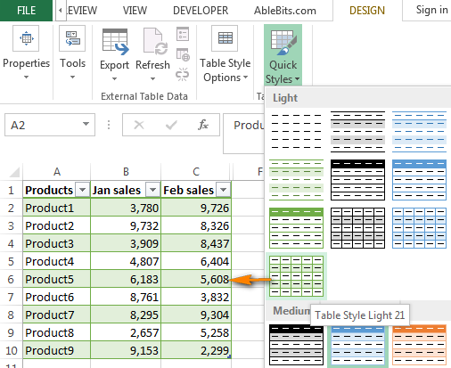
Ever find yourself staring at a spreadsheet full of data, struggling to make sense of it all? The rows blend together, making it hard to distinguish key details. Maybe you’re struggling to analyze your budget, track inventory, or follow a complex project timeline. No matter the task, a simple formatting trick can make your data much easier to read: color-coding your rows. With just a few clicks, you can create a visual rhythm that guides your eyes and highlights important information, making your Excel experience far more efficient and painless.

Image: www.coldfrontservices.com
Coloring every other row in Excel is a surprisingly versatile technique. It can quickly organize your data, making patterns and trends easier to spot. It can also add a touch of professionalism and make your spreadsheets more visually appealing. But beyond the cosmetic benefits, it truly enhances your data analysis experience. So, let’s dive into the world of conditional formatting and discover how to effortlessly transform your spreadsheets into vibrant, organized, and information-rich tools.
The Basics of Conditional Formatting
What is Conditional Formatting?
Conditional formatting is a powerful Excel feature that allows you to apply formatting, like changing font color, background color, or adding borders, based on specific criteria. Imagine a set of rules that dictate how a cell’s appearance changes based on its content. For example, you could set a rule to automatically turn a cell red if its value is below a certain threshold. Conditional formatting is the magic behind those dynamic changes, allowing you to create visually impactful spreadsheets that react to your data.
Applying Conditional Formatting in Excel
To color every other row using conditional formatting, we’ll use a technique called “Formula-based formatting.” This method gives us the flexibility to define custom rules for highlighting our data. It’s like giving Excel an instruction manual for how to color the rows.
Here’s a step-by-step guide to applying conditional formatting to color every other row in Excel:
- Select the range of cells you want to format. Be sure to select all your data, as this determines the scope of the rule you’re about to create.
- Navigate to the “Home” tab on the Excel ribbon. Click on the “Conditional Formatting” dropdown in the “Styles” section.
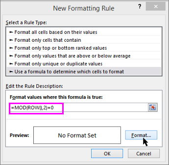
- Choose “New Rule…”. A dialog box will appear, allowing you to create your formatting rule.
- Select “Use a formula to determine which cells to format.”
- In the “Format values where this formula is true:” box, enter the formula: “=MOD(ROW(),2)=0”
- Click the “Format…” button.
- Choose the desired fill color for your even-numbered rows. You can also change the font color and add other formatting options.
- Click “OK” twice to exit the dialog boxes.

Image: support.office.com
Understanding the Formula
Let’s break down the formula “=MOD(ROW(),2)=0.” This formula utilizes the MOD function, which returns the remainder after a division operation.
- ROW(): This function returns the row number of the current cell.
- MOD(ROW(),2): This calculates the remainder when the current row number is divided by 2.
- =0: This condition checks if the remainder is equal to 0. If it is, it indicates that the row number is even.
By setting the condition to “=0,” we’re telling Excel to apply the color formatting only to the rows with an even number. This formula is the backbone of our rule, ensuring that every other row receives the chosen color.
Beyond the Basics: Fine-Tuning Your Formatting
Coloring Odd-Numbered Rows
If you want to color every other row, but prefer to start with odd-numbered rows, simply adjust the formula to “=MOD(ROW(),2)=1”. This minor change will highlight the odd rows instead of the even ones.
Adding Visual Variety with Multiple Colors
Want to add a bit more creativity and readability to your spreadsheet? You can use multiple colors by adding additional rules. When selecting “New Rule…” from the conditional formatting dropdown, you can add multiple rules for different color patterns, such as color-coding every third row or using a red-green alternating pattern.
Using Conditional Formatting for More Than Just Colors
Remember, conditional formatting isn’t just for colors. You can create rules to change font colors, add borders, and even apply custom formatting based on your data. For example, maybe you want to highlight cells containing specific keywords, or use italicized text to emphasize important values. The possibilities are endless, expanding the power of conditional formatting to create dynamic and informative spreadsheets.
Real-World Applications and Advanced Uses
The ability to color every other row is incredibly versatile in practical spreadsheets. Here are some examples of how you might use this technique:
- Budget analysis: Color-coding your budget categories can help you visualize where your money is going, making it easier to identify areas where you might save or spend more.
- Inventory tracking: Highlight low-stock items to ensure you reorder them in a timely manner.
- Project management: Color-code tasks or milestones to prioritize key activities and visualize workflow progress.
- Data analysis: Use colors to group similar data points, making patterns and trends more readily apparent.
Integrating Color-Coding with Other Excel Features
You can further enhance color-coding by integrating it with other Excel features:
- Filters: Apply color-coding to individual rows within filtered data to highlight specific results.
- Pivot tables: Use conditional formatting to color-code rows within a pivot table, creating visual representations of trends and relationships within your data.
- Data validation: Combine color-coding with data validation rules to quickly flag invalid data entries, ensuring data accuracy.
Excel How To Make Every Other Row Color
Making Your Spreadsheets Stand Out
Color-coding every other row may seem like a simple formatting trick, but its impact on your spreadsheets can be significant. By adding visual organization to your data, you’ll improve readability, make it easier to spot trends, and even enhance your creative potential.
Don’t be afraid to experiment with different color palettes and formatting styles. Your goal is to create visually appealing spreadsheets that not only convey information effectively but also reflect your personal style. Excel offers a wide range of customization options, empowering you to turn your data into dynamic and impactful stories.


